Filtering and Downsampling

By Sven Leach (last updated: not yet)

Filtering: Background

One of the major challenges of brain science is that measurements are contaminated by noise and artifacts. These may include environmental noise (e.g. electrical line noise), instrumental noise, or physiological noise (e.g. signal sources within the body that are not of interest, such as heart beat). Filters are commonly used to reduce noise and improve data quality. This is possible in case the noise occupies a spectral region other than your signal of interest (e.g. line noise at 50 Hz and slow delta oscillations during sleep at around 1 Hz). In this case the filter can attenuate the noise in the data and leaves the signal of interest (i.e. brain signal) “untouched”. In practise, as everything in life, this dichotomy is not perfect, meaning that the signal of interest is also affected by the filter, but (usually or hopefully) to a minimal extend.

A filter for signal processing is not that different from a coffee filter: it removes the unwanted parts (coffee grounds or *artifacts*) and lets the wanted parts pass (water with coffee flavour or *brain signal*).

Another way to think about filters

Every signal can be thought of as built up from a large number of sine and cosine waves with different frequencies. A filter now attenuates the signal for each of its frequencies differently. Ideally, the passband frequencies (the frequencies of interest) of the signal will be passed unchanged from input to output. The stopband frequencies (noise), however, should be attenuated at the output of the filter.

Filter applications

For example, a direct current (DC) component or slow fluctuation may be removed with a high-pass filter (a high-pass filter leaves high frequencies in the signal, they “pass” the filter), unwanted high-frequency components may be removed by smoothing the data with a low-pass filter (low frequencies are left in the signal, they “pass” the filter), and power line components may be attenuated by a notch filter at 50 or 60 Hz (only a specified frequency range is filtered out). A filter that removes low and high frequencies at the same time is called a band-pass filter (a specified frequency band, such as 10-20 Hz “passes” the filter).

Examples of high-pass, low-pass, band-pass & notch filter.

Below you can see the four different filter types and how much these specific examples attenuate certain frequency ranges. The attenuation can be visualized on a logarithmic scale, usually decibels (dB), or on a linear scale, usually percent (%). Zero attenuation means that those frequencies are not touched. Positive attenuation means that frequencies become stronger. Negative attenuation refers to a reduction in amplitude of those frequencies. Those plots show the attenuatoin on a logarithmic scale. As such, an attenuation of -40 dB is not double as strong as -20 dB (as it would be the case on a linear scale), but actually 100x stronger.

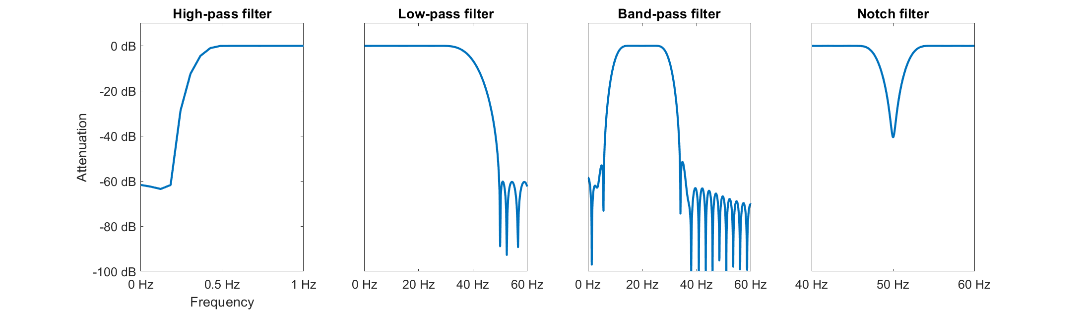FIGURE CAPTION???

Examples of filtered EEG.

Here are two examples of how filters can reduce unwanted features of the EEG. On top of the following figure you can see a direct current (DC) component that shifts the signal away from zero by a constant. Correct EEG signal should oscillate around zero. Due to the DC component, we see values of up to 20.000 \muV. Additionally, over 8h of recording, the data contains a slow negative drift which results in a difference of around 10.000 $\mu V$ when comparing the beginning to the end of the night. Both unwanted features can be removed by a high-pass filter.

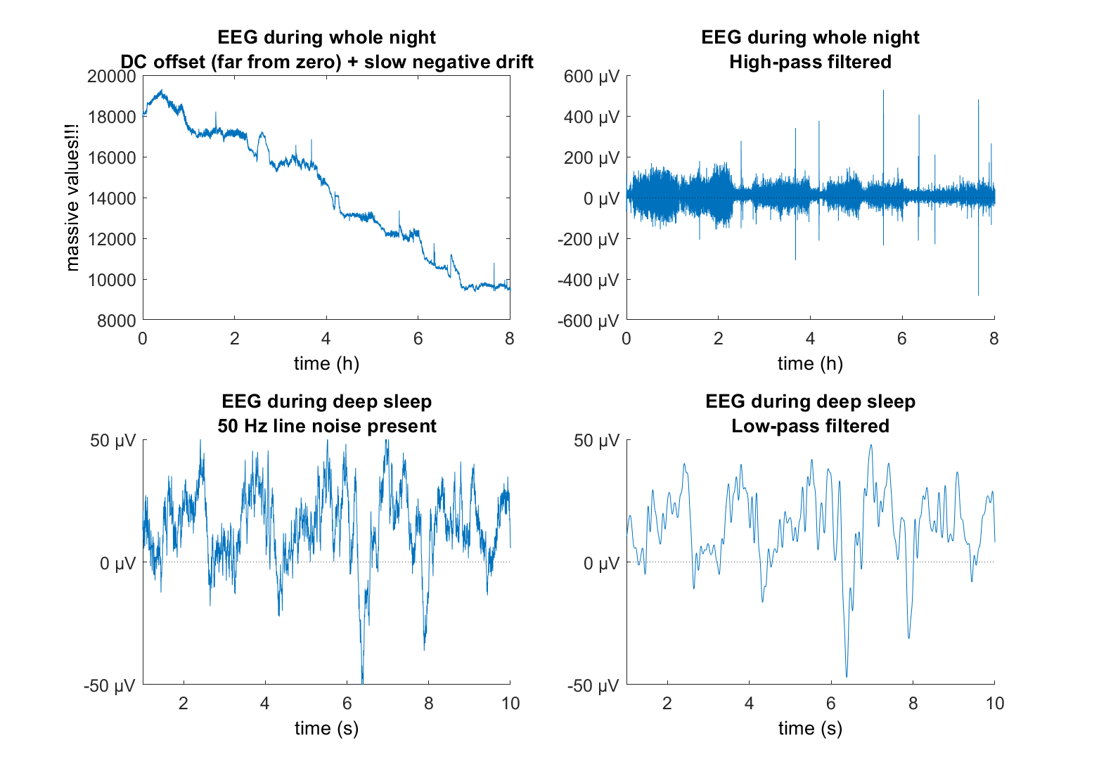FIGURE CAPTION???

On the bottom of the figure you see a very common artifact in EEG data: 50 Hz (EU) or 60 Hz (USA) line noise. Electrical devices and cables transport electrical power which alternates 50 or 60 times per second (alternating current). This 50 or 60 Hz activity can show up in the EEG, especially where the electrode does not make good contact, or where there are simply too many cables and electrical devices around. It is commonly reduced by using a 50 Hz notch or an appropriate low-pass filter.

What Is a Filter?

For many of us, a filter is “a thing that modifies the spectral content of a signal”. Mathematically, a filter is an operation that produces each sample of the output waveform y as a weighted sum of several samples of the input waveform x. This operation is called convolution and wonderfully explained in this youtube video.

The exact way of how a filter “changes” the data is defined by it’s impulse response function (that is, the output in response to an impulse). Some filters may smooth the input waveform, others may enhance fast oscillations. There are numerous different filter types (such as window-based FIR filter, butterworth IIR filter, chebyshev IIR filter, etc.) and different ways to implement those filters into software (i.e. by using toolboxes such as EEGLAB or designing your own filter either by hand or with helpful add-ins, such as MATLAB’s filter designer. Respectively, there is considerable body of theory, methods, and lore on how best to design and implement a filter for the needs of an application.

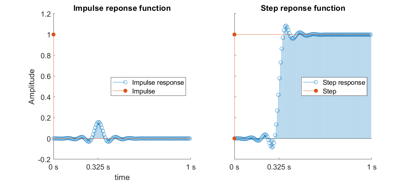FIGURE CAPTION???

FIR vs. IIR filters

One of the most important distinction of filters is whether a filter is an Infinite Impulse Response (IIR) or a Finite Impulse Response (FIR) filter (their mathematical equation decides to which category a filter belongs, but we will elaborate on equations here). Conceptually, as the name suggests, these filters can be differentiated by their impulse response. An FIR filter has a finite effect on an impulse, meaning that the induced ringing will stop completely with time. The ringing induced by an IIR filter, on the other hand, is indefinite, meaning that the ringing will be reflected in the whole recording (while this is technically true, the ringing becomes unconsiderably small with time as well).

The ringing introduced by both the FIR and IIR filter is bigger, the larger the filter order. While the ringing of the FIR filter is strictly limited in time (determined by the filter order), the ringing of the IIR filter is comceptually indefinite (even though you see here that is also quickly approximates 0). For FIR filters, the filter affects the signal for exactly one sample point longer than their filter order, so in our example 21 and 61 sample points (which translates to 0.17 s and 0.49 s at a sampling rate of 125 Hz).

In practice, IIR filters have the advantage that they are considerably faster due to their low filter order (somewhere around 1 to 10). FIR filter need a higher filter order (somewhere around 100 to 1000) to achieve the same attenuation of frequencies as a respective IIR filter. However, an IIR has nonlinear phase and stability issues. It is a bit like the fable of the tortoise and the hare. The FIR filter is like the tortoise in the race – slow and steady, and always finishes. The hare is like the IIR filter – very fast, but sometimes crashes and does not complete the race. This is why, generally speaking, FIR filters are prefered whenever computation time allows to do so (such as offline analyses, so analyses on data that are already recorded). There are domains, however, such as real-time processing, where computation speed is ciritical, which is why you will usually find IIR filters there (the algorithm on our SleepLoop device is such an example, it uses IIR filters).

	Infinite Impulse Response (IIR)	Finite Impulse Response (FIR)
Copmutational speed	Fast (Low filter order)	Slow (High filter order)
Phase delay	Not constant (across frequencies)	Constant (across frequencies)
Stability	Sometimes	Always

Both FIR and IIR filters attenuate unwanted frequencies better at a larger filter order. The larger filter order comes, as you have seen above, at a price of stronger smearing. Note that the filter order of IIR filters are always smaller then of FIR filters, which speeds them up considerably.

Phase shift

Important in our line of research is at what phase of a slow wave an auditory stimulus was presented. Some filters introduce a phase shift which is different for each frequency in the signal. When analyzing data to which we introduced a phase shift by the type of filter we applied, we would assume a completely wrong phase precision of our stimulation algorithm. This is why zero-phase filters are especially important to us. FIR filter change the phase of the signal linearly (or evenly) for all frequencies, so that it can be easily corrected. In practice, you can either use the function firfilt() together with an FIR filter. It applies the filter once and corrects for the introduced linear phase shift. The function is part of the EEGLAB toolbox. If you use an IIR filter, you should use the function filtfilt() to filter your data. This function applies the filter twice in both directions (also called two-way filtering) and by that reversing any introduced phase shift.

FIGURE CAPTION??? one radian is 180/π degrees (~ 57.3°). In figure xx you can additionally see that the linear phase shift of the FIR filter shifted the impulse response 0.325 s to the future. The shift can be easily inferred from the filter order of the filter, which the firfilt() function does in order to correct for this shift.

Consequences of two-way filtering

While filtfilt() is a convenient option to circumvent the problem with non-linear phase shift of IIR filters, you should be aware of the consequences. What you do is filtering the data twice, meaning that you also double the length of the impulse response (biggrt smearing in time of original samples on the filtered output) and the attenuation of your data: frequencies which were attenuated at 60 db before are now attenuated at 120 db. This, of course, needs to be correctly reported in your publication. While this seems to be even a wanted side effect, be aware that any modifications to your pass band (your frequencies of interest) also doubles in magnitude. Conceptually, two-way filtering should be avoided whenever possible (why should you repeat a processing step twice, right?).

Some terminology

The cutoff frequency separates passband and stopband of the filter and always lies in the transition band. This is the value that is most likely to be reported when a filter is applied during the signal processing, but it is not sufficient to characterize the filter. Different definitions of cutoff frequency are used: −3 dB (half-energy) cutoff (common for IIR filters; see Section 2.7 below) and −6 dB (half amplitude) cutoff (common for FIR and two-pass IIR filters). Therefore, cutoff frequencies should always be reported together with the definition used. Optimally, the cutoff frequency should separate signal from noise components in the frequency domain. To avoid unwanted signal distortions, it is essential to select the cutoff frequency so that no spectral component of the signal is attenuated but as much noise as possible is removed.

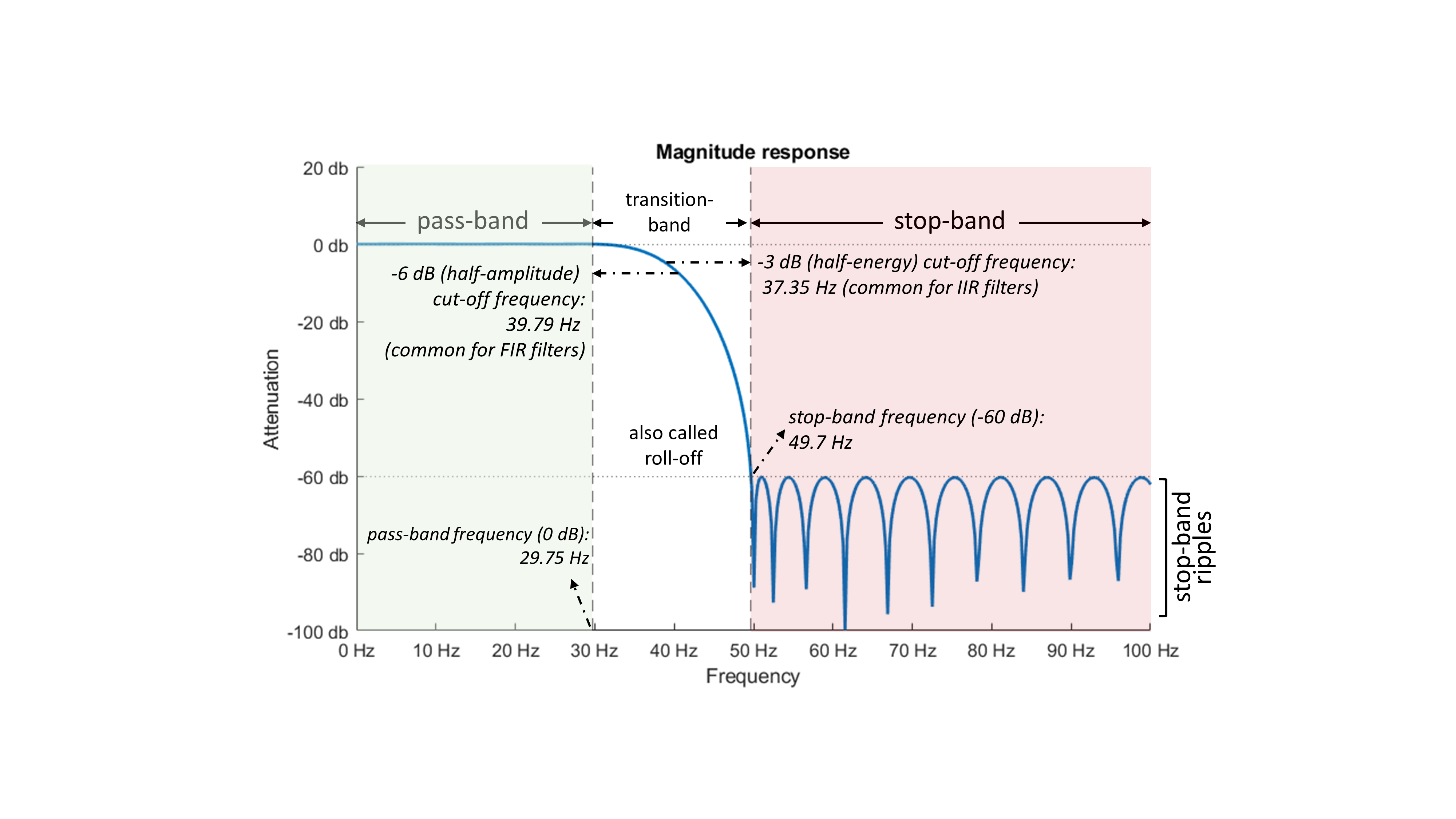
Stop-band ripples describe the phenomenon that frequencies in the stop-band are not all evenly attenuated at, let’s say, -60 db, but that the attenuation fluctuates over frequencies. Hence, while the example filter attenuates all frequencies in the stop-band for at least -60 db, some frequencies are attenuated even stronger. As this waxing and waning in attenuation resembles ripples, it is commonly referred to as stop-band ripples. Similarly, pass-band ripples describe the phenomenon that not all frequencies are perfectly untouched in the pass-band, but that some are attenuated, while others are even increased. The strength of this unwanted attenuation & amplification in the pass-band is determined by the maximal passband deviation. With a passband deviation of, for example, 0.01, the filter output does not amplify or attenuate the signal by more than 1% in the passband (0.086 dB, note that in MATLAB passband ripple is defined as peak-to-peak ratio: rp = 20 log10((1 + 0.01) / (1 − 0.01)) = 0.174 dB). While the pass-band ripple should be as low as possible, lower pass-band ripples requier higher filter orders, which again lead to longer impulse responses. Thus, pass-band ripples should not be chosen too small. For instance, passband ripple of 0.002–0.001 (0.2%–0.1%) are reasonable values for many ERP/F applications.

An important goal of neuroscience is to determine causal relations, for example, between a stimulus and brain activity, or between one brain event and another. If a filter is causal, the filter output depends only on past and present samples of the input. If a filter is acausal, the filter output also depends on future samples of the input. Basically anytime you use the function filtfilt() to correct for the introduced phase shift of an IIR filter, each sample in the filtered output signal is computed from preceding (past) and following (future) samples of the unfiltered input signal. In any scenerio where you want to compare the EEG at baseline before an event occured, the event now also contributes to the EEG at baseline, which is usually not wanted at all. Only a causal filter would evade that problem. The step response of a causal filter does not exhibit signal changes due to the step (for example smoothing or ringing) before the onset of the step in the filter input

plot..causal..filter..

Example on how to build a filter

Within MATLAB alone there are numerous ways on how to build and run a filter. The easiest way is probably to use functions provided by external toolboxes, such as eegfilt() or pop_eegfiltnew() from the EEGLAB toolbox or ft_preproc_lowpassfilter() from the FIELDTRIP toolbox. You typically just give those functions the cut-off frequencies of your choice and they will design and apply the filter for you. When using functions from toolboxes, you can rely on the filterdesign of the people who designed those toolboxes. While this is great for the start, it is usually a blind approach as you do not need to investigate the impulse response function of the filter, meaning that you do not know how well it performance in the frequency vs. time domain.

A more sophisticated and effortful approach, which also requires some knowledge about how filters work, is to design your own filter. MATLAB provides great functionality to design and test a filter rather easily. When executing the command filterDesigner, MATLAB’s filter Designer opens up which is a visual GUI to design your own filter with various types of specifications. An example of such a filter that I build with MATLAB’s filter Designer is this 0.5 Hz high-pass filter.

srateFilt    = 500;   % sampling rate (Hz)
PassFrq      = 0.5;   % pass-band frequency (Hz)
StopFrq      = 0.20;  % stop-band frequency (Hz)
PassRipple   = 0.02;  % pass-band ripple
StopAtten    = 60;    % stop-band attenuation (dB)
HiPassFilt   = designfilt('highpassfir','PassbandFrequency',PassFrq,'StopbandFrequency',StopFrq,'StopbandAttenuation',StopAtten,'PassbandRipple',PassRipple,'SampleRate',srateFilt,'DesignMethod','equiripple');

Once the filter is built, you can investigate the filter by visualizing it’s impulse reponse using impz(HiPassFilt, filtord(HiPassFilt)). This will tell you how the filter will affect an impulse (all zeros expect for the first sample point, which is 1). From the impulse response you can for example see how much your filter “rings” in the time domain, meaning how much the first datapoint is smeared out into the past and/or future in the form of oscillations that become smaller after time.

What can go wrong?

Unortunately, the use of filters raises many concerns, some serious, others merely inconvenient. Therefore it is important to understand them, and to report enough details that the reader or listener too fully understands them.

An obvious concern is loss of useful information suppressed together with the noise (a filter does not distinguish between brain signal and noise, it only distinguishes between frequencies). Slightly less obvious is the distortion of the temporal features of the target: peaks or transitions may be smoothed, steps may turn into pulses, and artifactual features may appear, such as response peaks, or oscillations (“ringing”) created de novo by the filter in response to some feature of the target or noise signal. The morphology of these artifacts depends on both the filter and the brain activity. Most insidious, however, is the blurring of temporal or causal relations between features within the signal, or between the signal and external events such as stimuli.

How to report

As filters can distort the signal, it is extremely important to thourougly report the filters you have used so that the reader can form an opinion about possible effects of filtering. In short, you are save when you report

The filter type
The filter order
Frequency parameters
Whether it was applied in one or both directions (filtfilt)
Advanced: include a plot of the impulse (or step) response function

Alternatives

Depending on the usecase of your filter, there may be better alternatives. For the example, if the high-pass filter is required merely to remove a constant DC offset, consider subtracting the overall mean instead. If there is also a slow trend, consider “(robust) detrending” rather than high-pass filtering. Detrending involves fitting a function (slowly varying so as to fit the trend but not faster patterns) to the data and then subtracting the fit. Suitable functions include low-order polynomials. Like filtering, detrending is sensitive to temporally localized events such as glitches; however, these can be addressed by “robust detrending” (de Cheveigne et al, 2016, de Cheveigne´ and Arzounian, 2018)

Downsampling

Downsampling reduces the sampling rate of your data to improve processing speed and to save disc space. We usually record EEGs with a sampling rate of 500 Hz, meaning that we record 500 sampling points per second.

In case one is only interested in oscillations around, let’s say, 0.5 to 40 Hz, this is an information overload. Defined by the Nyquest theorem (LINK), a 40 Hz oscillation can be represented in the data with a sampling frequency of 80 Hz (better 120 Hz). You could therefore downsample the recording to produce an approximation of the sequence that would have been obtained by sampling the signal at 125 Hz. It is generally better to choose a sampling rate which is a multiple of the original samplring rate (4 * 125 = 500), as no “new” datapoints need to be estimated. Downsampling at, let’s say, 128 Hz would require interpolating non-existing data points.

Lastly, it is important to say that you should always low-pass filter before downsampling (aliasing problem (LINK)).

Example Intro

We just love the 2-process model by Alexander Borberly:

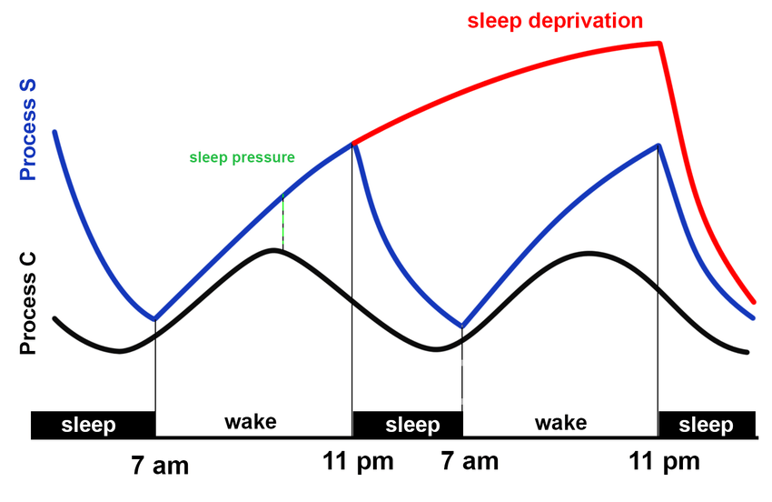
I’m not going to bother explaining it, so just look here.

If you can’t do something fancy in Markdown, you can just write in HTML: Just Google It!

But! What if someone here already presents it? Well I can just link it like so. In case you didn’t notice, there’s a cute little menu on the left, but it will only write up to three ### pound signs.

Subpoint to the intro

Bulleted
List

Numbered
List

Example Code

Var1 = 3;
Var2 = 5;

Result = Var1*Var2;

Now just replace the numbers in Var1 and you can do math!

Example data

If you’re really fancy, you can add a table:

Row Names	Data
First row	Lots of data
Second row	More data

A = 3;
B = [1 2 3];
F = plot(B,A);

close all

The m makes it matlab colored